
.png)

Objectives
The objectives of this chapter is to study price- output decisions under non-collusive oligopoly. While going through this chapter, you will study about various models of non-collusive oligopoly and analystical difficulties in oligopoly market.
We will discuss under this
1) Chamberlin's Model
2) Kinkd Models of Oligopoly
3) Stackelberg's Duopoly Model
Chamberlin's Model
Chamberlin questioned the illogical assumption in all the three classical models of oligopoly discussed above, namely, that the producers do not learn from their experience even when their assumption regarding the behaviour- reaction of the rival producers is falsified again and again. These models imply that the oligopolists are so short-sighted that they are unable to recognise their mutual dependence. Chamberlin does away with this unrealistic assumption and instead assumes that oligopolists are sure to recognise their mutual dependence either intuitively or as a result of experience.
Thus the distinguishing feature of Chamberlin's model of oligopoly is that it is securely based on the assumption that the duopolists or the oligopolists, as the case may be recognise their mutual dependence. Therefore, in his model, the oligopolist does not assume that his rivals will continue to stick to their output or price or both regardless of what he does to his own output or price or both. Instead, he perceives that any move by him to gain advantage at the expense of his rivals will be retaliated. If any individual oligopolist thinks of lowering his price he can easily see that the number of firms in the “industry” or “group” being very small particularly in the case of duopoly, the adverse effect of his price-cutting on the sales of his rivals will be significant. Therefore, he will foresee that his rivals will not stick to their current price and output but will strike back by lowering their prices.
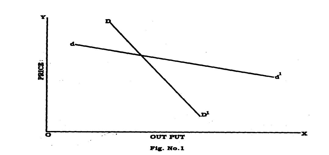
On account of this perception he can easily see that his own sales, as the result of price-cutting, will increase not along the elastic sales curve dd' of Fig. I above but along the inelastic sales curve DD' of this Fig. 1. Such a result of a price cut by any of the oligopolists is not likely to increase his profits. Hence, the oligopolists recognising their mutual dependence, will avoid any engagement in a price war one another.
The same recognition of mutual dependence which prevents the oligopolists from indulging in price cutting competition will induce them to fix their price at the level which would have prevailed under monopoly. Of course, this is based on the heroic assumption that the cost curves of the oligopolists are identical and such that, when added together, will become identical with the cost curves of single monopolists. The equilibrium output of the “industry”or the “group”, in that case, will be the same as the equilibrium monopoly output under a single monopolists and this total output will be equally shared by all the oligopolists. It may be thought that the solution of equilibrium problem under oligopoly as suggested by Chamberlin and explained above points towards “collusion” among the oligopolists. But Chamberlin argues that the monopoly arrangement among the oligopolists that results in his model is not the result of any collusion among them. It rather results from the oligopolist's intuition or business sense or their experience gained through some earlier price war.
However, regardless of the contention of Chamberlin his model is not a model of a purely non-collusive oligopoly. There may not be in his model an open agreement among the oligopolists on the monopoly arrangement, but there is a tacit agreement all the same.
We have already pointed out the basic weakness of the classical models, namely, that they implicitly assume that oligopolists do not learn from their experience. That they are permanently short-sighted and therefore fail to recognise their mutual dependence. Chamberlin's model does not suffer from this failing but his model is not a model of a genuine not-collusive oligopoly. But there is another more fundamental weakness which not only Chamberlin's model but also a number of other models share with the classical models.
All these models are based on the assumption of perfect knowledge and they rule out uncertainty. As soon as we introduce uncertainty into a model of oligopoly, the analysis of equilibrium under oligopoly becomes even more complicated.
This has led some mathematical economists like Von Neumann and Morgenstern to suggest that laws governing the behaviour of oligopolists resemble not to the laws of physics, from which the technique of equilibrium analysis has been borrowed by the economists, but the laws governing the outcome of games and wars which involve strategies and counter-strategies.
Kinky Models of Oligopoly
The kinky models of oligopoly are described so because they postulate the demand curve or average-revenue curve facing an oligopolist as a curve which has a kink in it at the current level of price as shown in Fig. 4 below. OP is the current price, the demand curve (AR curve) facing the oligopolist is DD' which has a kink at k corresponding to the current price P. Its
companion marginal-revenue curve is MR curve which too has rather two kinks in it at A and B. The solid vertical regiment AB over it is described as
the discontinuity gap which is due to the sudden change in the elasticity of the demand curve from just above

Note that the kinks A and B in the marginal-revenue curve MR as well as the discontinuity gap AB are exactly below the kink K, that is, if you extend the discontinuity gap AB. vertically upwards, it will pass through K. This model
stipulates that the cost conditions of the oligopolist are such that his marginal cost curve MC cuts the marginal-revenue curve in its discontinuity gap marginal revenue is the profit-maximising output and OP is the profit-maximising price. The oligopolist in this model does not experiment with price-output changes. It is because he is assumed to expect a retaliation by his rivals, if he reduces his price and consequently his sales are expected to increase along the less elastic portion of his demand (sales or average-revenue) curve.
Therefore he will not expect to increase his profits by a cut in his price. He will not experiment with an increase in his price either, precisely because int this case he does not expect his rivals to follow him suit. If our oligopolist raises his price, it does not harm his rivals but, on the contrary, is beneficial for them. Hence they are not expected to match any increase in price that out oligopolist may effect. And, the portion of out oligopolist's demand curve above the kink being highly elastic, any increase in his price will reduce his sales
proportionately much more and thus reducing his total revenue too. Hence he will not increase his price. Thus the tendency would be to stick to the current price and output. This explains the rigidity or stickiness of prices under oligopoly. It can be seen from Fig. 4 above that even when the costs of the monopolist increase or decrease and in consequence of which his marginal cost curve shifts up or down, the equilibrium price and output of the oligopolist will not change, provided the shifted MC curve continues to cut the MR curve in its discontinuity gap.
Paul Sweezy has suggested that the obtuse-angled demand curve as postulated in the model of Fig. 4 above is peculiar to periods of depression when there develop buyer's markets because then in most of the industries demand lags behind supply, in such a situation any cut in price by any one of the oligopolists is sure to be retaliated with similar cuts by the other firms also, while any increase in price by one will not be followed by others.

But, argues Sweezy, during periods of boom and prosperity there develop seller's markets as then demand moves ahead of supply. Therefore
producers do not find any difficulty in selling. In this condition a cut in price by one will not be followed by others. This means that the demand curve below the current price will be elastic. On the other hand, an increase in price by any one will be followed by others which means that the portion of demand curve above the kink will be inelastic. This behavioural assumption read to boom period will give a reflex-angled kinked demand curve like the one in Fig. 5 this type of demand curve can also be derived form Fig. 1 by continuing the
portion of inelastic demand (sales) curve DD' above the point of intersection between DD' and dd' with the lower portion of the elastic of dd.' curve.
In this case also the equilibrium price will be OP and equilibrium output PC which will tend to be rigid so long as the marginal cost curve continues to cut the marginal revenue curve in the discontinuity gap.
It is sometime observed that kinky models of oligopoly explain the rigidity of prices under oligopoly but they do not explain how equilibrium price is determined under oligopoly. This observation is not quite correct because as we
have seen above the kinky models are consistent with the conventional profit- maximising principle of price determination, it is, though a different matter, if the current price is made to be determined by some other principle such as the
“cost-plus” or “mark up” or full-cost principle and then kinky models are relied on to explain the rigidity of prices. We shall consider the full-cost principle of Hall and Hitch in the lesson on the Marginalist Controversy.
Stackelberg's Duopoly Model
The profit of each duopolist is generally, taken as a function of the output levels of both, i.e.
π1=h1(q1,q2) and
π2=h2(q1,q2)
The Cournot solution is obtained by maximising π1 with respect to q1 assuming and keeping q2
as constant. Similarly, π2 is calculated with respect to q2,where q1is assumed to be constant. This means each firm might make certain assumptions about its rival's response. To the extent the firms make erroneous assumptions about each other's response will not be called an
improvement over the Cournot's model of duopoly.
An attempt regarding the variation in the sets of assumptions is contained in the analysis of leadership and followership given by Heinrich Von
Stackelberg, a German economist. A follower obeys his reaction function and sets his output level that maximise profit given the quantity decision of his rival to whom he regards his leader. But a leader is supposed to obey his reaction function. He assumed that his rival acts as a follower, and maximises his profits, given his rival's reaction function. Each duopolist determines his
maximum profit from both leadership and followership and tries to play the role which yields the still larger maximum. In such a situation four outcomes are possible : (1) I (duopolist) desires to be a leader, and II a follower; (2) II desires to be a leader and I a follower; (3) Both desire to be leaders; or (4) both desire to be followers.
Stackelberg tried to make an improvement, though implicit, in Cournot's model. He assumes that one duopolist is enough sophisticated to recognise
that his rivals acts on the Cournot's assumption. It enables the sophisticated duopolist to determine the reaction curve of his rival and incorporate it in his own strategy for maximum profit. It can be shown with the help of a diagram. The isoprofit curves and the reaction functions of the duopolists have been shown in figure 6. Suppose there are two firms A and B. If firm A is sophisticated oligopolist it will assume that firm B will act according to its own reaction curve. This presumption would allow firm A to select its own
production level which provides it the maximum profit. In the fig. 6 this has been shown by point a which is on the lowest possible isoprofit curve of A.
This indicates the maximum profit A can earn given B's reaction curve. Here firm A acting as a monopolist will produce XA and firm B will react by
producing XB on the basis of its own reaction curve. The oligopolist who acts on Cournot's assumption becomes followers and the sophisticated one becomes the leader. The follower becomes worse off in comparison to
Cournot's equilibrium. It is because with this level of output he faces an isoprofit curve which is relatively, at a longer distance from his axis.
Suppose, if B is the sophisticated leader, it would like to produce X-B which is indicated by point b on A's reaction curve and which provides the
maximum possible profit to B in the face of its isoquant map and A's reaction curve. In this case firm B, being leader would earn higher profit than A, as compared with Cournot's equilibrium solution.

But, there can be a situation where both firms are sophisticated. In this situation both will try to act as leaders and the situation is termed as
stackelberg's disequilibrium. Due to the actions of the both either there would be a price war until one of the firms accepts its defeat and starts acting as a follower or there can be collusion between the two firms. In this case, the collusion point would be on (or nearer to) the Edgeworth contract curve where both the firms obtain higher profits. It implies that naive behaviour does not pay and the firms should realize their interdependence. If firms do not take into consideration the actions and reactions of each other, both will be worse off, due to the price war. Thus, it is by realising the other's reactions each firm can earn a higher lever of profit for itself. But, when the model is assessed critically, it is said that in a Cournot- type market situation the sophisticated duopolist bluffs the rival one, by producing level of output higher than the one that would be produced under the Cournot equilibrium. And also if the naive rival, sticks to his Cournot behavioural reaction style and being misled, produces less than what he would
have produced under the Cournot equilibrium.


No comments:
Post a Comment